Pick a split and a model version; the bar chart, the delta panel, and the per-version readout below all re-render from the committed numbers. The metric is locked to surface coverage: mep_recall is too sparse on the OOD set to compare meaningfully (most scenes capture 0 instances, so per-scene recall is mostly zeros). The honest read: the learned ranker alone never tops greedy_coverage; what ships is the hybrid (learned scores, top-K=12, then 2-step lookahead).
How it works: from a building to a scan
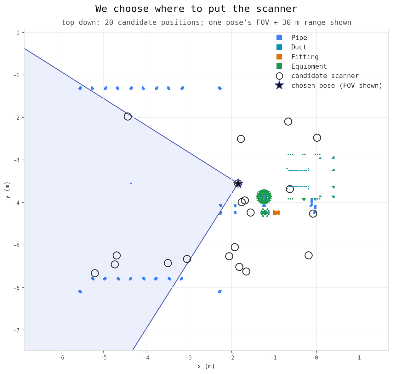
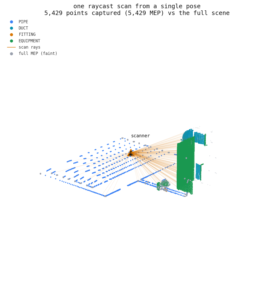
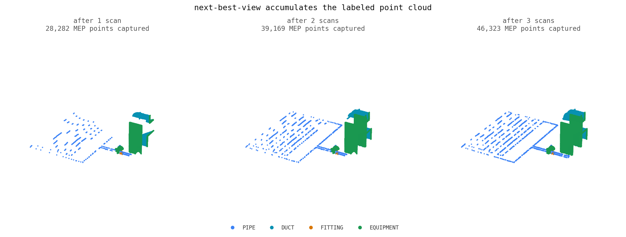
Before the interactive comparison, three pictures of the actual task: choose a pose, see what one scan captures, then watch coverage accumulate. recall@K=1 (the headline metric) is just how much of the hidden MEP the growing union of scans covers.
1. We choose where to scan. Top-down view of one building with 20 candidate scanner rings; we pick one pose (white star) and show its field of view out to the 30m range. The task is to decide, before scanning, which pose reveals the most hidden piping.2. What one scan captures. A single scanner pose (white triangle) fires rays to every reachable surface point; the bright points are the roughly 5,400 it captures, the faint grey points are the rest it cannot see from here. One viewpoint sees only a slice, which is why view selection matters.3. Coverage accumulates, one scan at a time. The point cloud after 1, 2, and 3 scans grows from roughly 28,000 to 46,000 captured points. recall@K=1 reads how much of the hidden MEP this growing union covers. A better policy gets there in fewer scans.
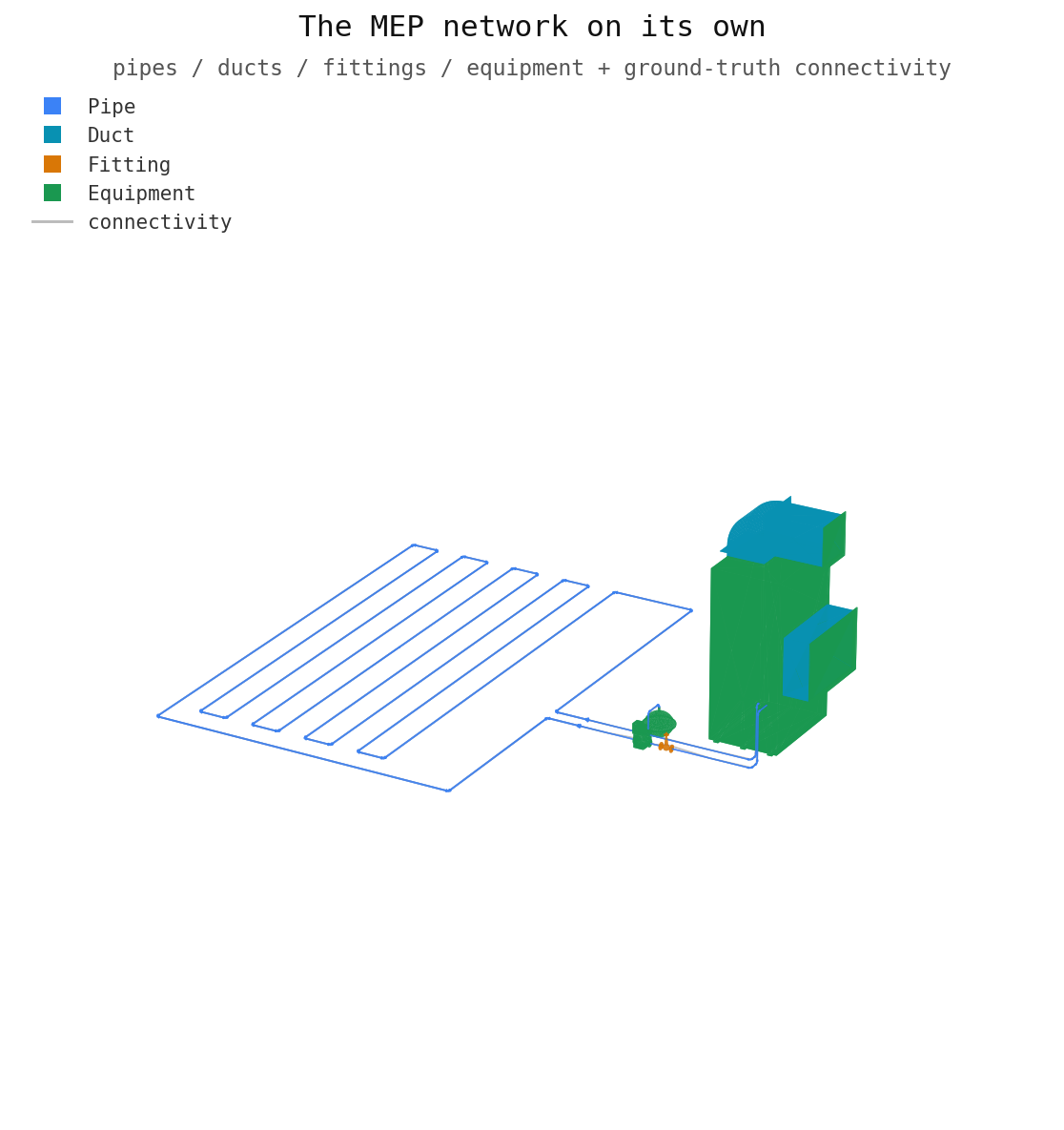
The network we are recovering. The MEP system on its own, building removed: the pipe grid, equipment block, ducts and fitting, plus thin lines for the 130 connectivity-graph edges joining physically-connected parts. This graph is the ground-truth network the method discovers, and the basis of the connectivity-aware edge_recall metric.
For the selected split and version, the hybrid minus three reference policies: greedy_coverage (the strongest classical heuristic), octomap_ig (the classical info-gain planner, Bircher et al., ICRA 2016), and greedy_lookahead_1 (the same 2-step lookahead the hybrid wraps, but with a true extractor and no learned prefilter). Combined SE = √(SEₐ² + SE_b²); σ = Δ / combined SE.
How to read it. Positive Δ and σ ≳ 2 means a real win at this sample size. The headline cross-split fact: hybrid beats octomap_ig by +5.4σ test_locked, +5.0σ held_out, +5.6σ OOD on surface coverage: every split, not one lucky cut. Note this is also where the honest story bites, on test_locked the hybrid still trails the strong greedy_coverage baseline.
Model version: training signal vs eval
The finding: higher training Spearman ρ does not buy eval wins. Three target-engineering bumps, namely v5 surface-target, v7_attn's 2.6M-param cross-attention head (ρ 0.13), and v7_k12's combined K2+0.1·K1 target, all regressed or no-gained. The one win, v7_realsynth (ρ 0.156), came from a realism-fixed procedural synth corpus, not a loss tweak. The bottleneck is corpus diversity, not target formulation.
Hybrid top_k: cost vs quality (documented sweep)
A static, documented finding (not re-derived here): how many of the model's top candidates you hand to the lookahead wrapper. More candidates means higher recall, but the true extractor runs on every pair, so extractor calls scale K². Quality saturates around K=12. Past that you pay quadratic compute for a recall that flattens (and dips at K=20).
recall@K=1 (surface) vs hybrid_top_k · extractor cost ∝ K² shown in the right column
Why K=12 is the shipped default. K=1 (0.443) is just the raw ranker: no lookahead. By K=5 (0.597) most of the gain is in; K=12 (0.615) is the knee; K=20 (0.598) actually regresses while costing ~2.8× the extractor calls of K=12. So the shipped hybrid_top_k=12 sits exactly at the cost/quality knee.
Why the learned ranker is a filter, not a policy
The ranker scores each candidate pose in isolation, so it learns the marginal MEP density of the scene cloud and not much else. The value of a pose depends on what the next pose will be: that joint reasoning is what the lookahead wrapper supplies. Left: the learned ranker prefilters candidates (top-K=12). Right: the classical lookahead does the 2-step joint search over that shortlist. Hybrid is both, in series.